import climetlab as cml
import datetime
import pandas as pd
import numpy as np
Show code cell content
# some helper functions
import matplotlib.pyplot as plt
import matplotlib.patches as mpatches
from matplotlib.lines import Line2D
from matplotlib.dates import num2date, date2num, DateFormatter
def prepare_seasonal_forecasts(seas):
seas_df = seas.to_dataframe()
seas_df = seas_df.drop(['lat','lon'], axis=1).reset_index()
# Since I don't want to plot every day of the forecast, filter weekly:
seas_df_w = seas_df[seas_df.time.dt.day.isin([2,9,16,23])]
leadtimes = seas_df_w.leadtime.dt.days.unique()
seas_df_w = seas_df_w.drop(["leadtime"], axis= 1)
seas_df_wf = seas_df_w.loc[(seas_df_w.time.dt.month >= 1) & ( seas_df_w.time.dt.month <= 12)].reset_index(drop=True)
seas_df_wf['time'] = pd.DatetimeIndex(seas_df_wf.time)
seas_df_wf['time'] = seas_df_wf.time.dt.strftime("%Y-%m-%d")
return seas_df_wf, leadtimes
def prepare_waterbalace(wb):
wb_df = wb.to_dataframe().reset_index()
wb_df.drop(["latitude", "longitude"], axis=1, inplace=True)
# wb_df= wb_df[(wb_df.time.dt.month >= 1) & (wb_df.time.dt.month <= 12) ]
wb_df['time'] = pd.DatetimeIndex(wb_df.time)
return wb_df
def prepare_climatology(cl, filter_time = ["2023-01-01","2023-12-31"]):
# daily climatology
cmean = cl.groupby("time.dayofyear").mean()
cmin = cl.groupby("time.dayofyear").min()
cmax = cl.groupby("time.dayofyear").max()
# drop 29th of February, extract timeseries
cmax = cmax.where(cmax.dayofyear != cmax.dayofyear[59], drop =True)
cmin = cmin.where(cmin.dayofyear != cmin.dayofyear[59], drop =True)
cmean = cmean.where(cmean.dayofyear != cmean.dayofyear[59], drop =True)
cmean["time"] = pd.date_range(*filter_time)
cmin["time"]= pd.date_range(*filter_time)
cmax["time"] = pd.date_range(*filter_time)
# cmean = cmean.isel(dayofyear=cmean.dayofyear <= len(cmean.time))
# cmin = cmin.isel(dayofyear=cmin.dayofyear <= len(cmin.time))
# cmax = cmax.isel(dayofyear=cmax.dayofyear <= len(cmax.time))
return cmean, cmin, cmax
def get_iseasonal_forecast(df, finit):
Fi1 = df[df.forecast_reference_time == finit]
Fi1_g = Fi1.groupby("time")
Fi1_g.groups.keys()
Fi1vals = []
for t in Fi1.time.unique():
vnew = Fi1.loc[Fi1_g.groups[t]]["dis24"].values
Fi1vals.append(vnew)
Fi1vals = np.stack(Fi1vals).T
xpositions = [date2num(datetime.datetime.strptime(t, "%Y-%m-%d")) for t in Fi1.time.unique()]
return Fi1vals, xpositions
def plot_seasonal(wb,
seas,
clims = [],
leadtimes = [],
clim_range_y = ["2000","2021"],
time_range = ["2022-01-01","2022-12-31"],
figsize = (15,5)):
finits = seas.forecast_reference_time.dt.strftime("%Y-%m-%d").unique()
wby = wb.time.dt.year.unique()[0]
wb_time = [date2num(i) for i in wb.time]
x_date = pd.to_datetime(
pd.date_range(*time_range,freq="MS"),"%Y-%m-%d")
timevals = pd.date_range(*time_range,freq="D")
cmeanvals,cmaxvals,cminvals = clims
fig, axs = plt.subplots(len(finits),1,figsize=figsize, sharex=True, tight_layout=True)
flierprops = dict(marker='o', markersize=2, linestyle='none')
medianprops = dict(color="red",linewidth=1)
boxprops = dict(color="black",linewidth=1)
# legend
red = mpatches.Patch(color='red', alpha=0.2, label='drier than average')
blue = mpatches.Patch(color='blue', alpha=0.2, label='wetter than average')
dots = Line2D([0], [0], color='black', linewidth=1, linestyle=':', label=f'{wby} discharge')
for i, f in enumerate(finits):
if i == 0:
axs[i].legend(handles=[red, blue, dots],ncols =3, bbox_to_anchor = [1,1.2])
fivals, xpositions = get_iseasonal_forecast(seas, f)
# climatology
axs[i].fill_between(timevals,cmeanvals,cmaxvals,color="blue",alpha=0.2)
axs[i].fill_between(timevals,cminvals,cmeanvals,color="red",alpha=0.2)
axs[i].plot(timevals,cmeanvals, linewidth=1, color="black",label = f"climatology {wby}", alpha=0.5)
# seasonal boxplots
axs[i].boxplot(fivals, positions=xpositions, widths=1.5,
boxprops=boxprops,
flierprops=flierprops,
medianprops=medianprops,
labels=leadtimes[:fivals.shape[1]]);
# water balance
axs[i].scatter(wb_time, wb.dis24, s=0.5, c="black")
axs[i].set_xlim([wb_time[0], wb_time[-1]])
axs[i].set_yscale("log")
axs[i].set_xticks(x_date)
axs[i].set_xticklabels(x_date.values, fontsize=10)
axs[i].xaxis.set_major_formatter(DateFormatter("%b"))
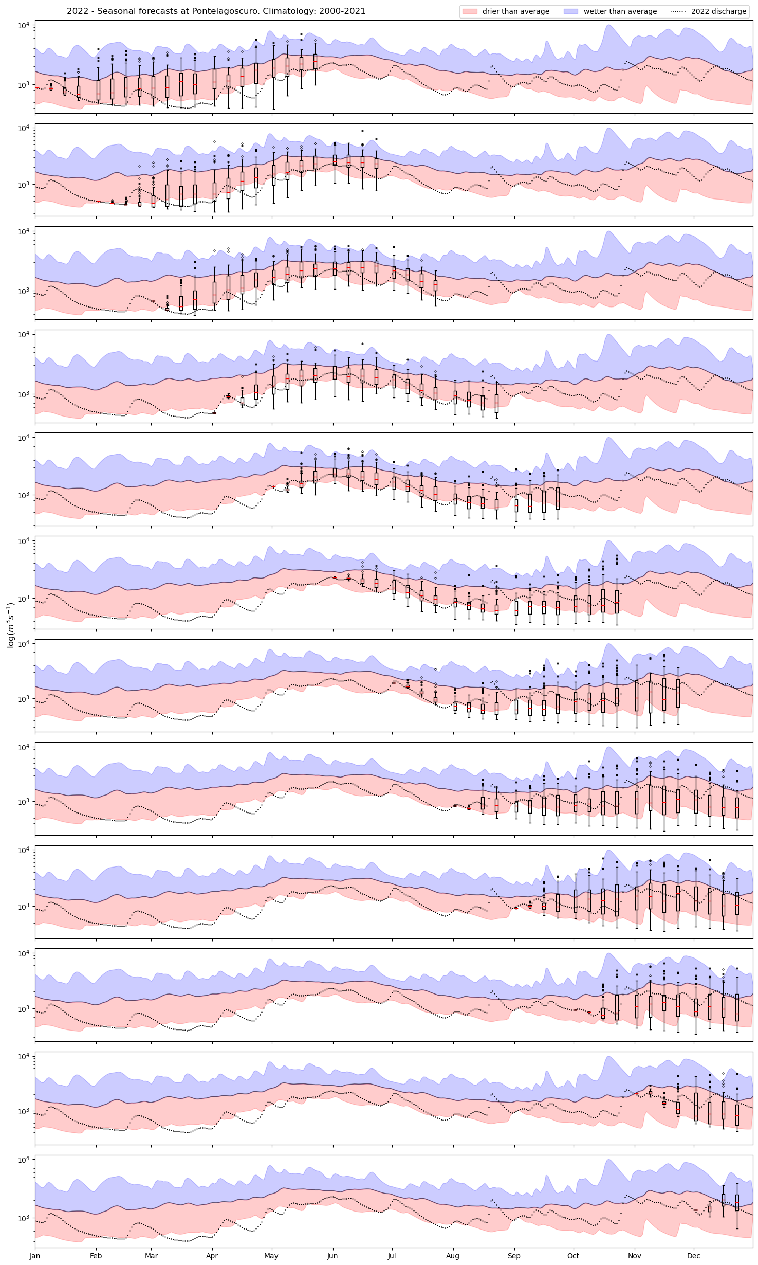
fig.suptitle(f"{wby} - Seasonal forecasts at Pontelagoscuro. Climatology: {'-'.join(clim_range_y)}", x=0.1, horizontalalignment='left', verticalalignment='top')
fig.supylabel(r'Discharge $\log (m^3 s^{-1})$')
fig.supxlabel(r'Time')
The intense drought on the Po river basin in summer 2022

The 2022 drought was one of the worst ever recorder on the Po basin (and not only there). The event was so severe that it was also reported in international newspapers, such as The Guardian: Quiet flows the Po: the life and slow death of Italy’s longest river
If you were in Northern Italy, it was an unbearable summer!
In 2022 the summer season started with water levels already in deficit due to below average winter and spring precipitation. The situation was alarming, and between one heatwave and the other, I decided to start monitoring the evolution of the water levels on the Po river, as the CDS, the CliMetLab API and this plugin make it quite easy to retrieve data not only for this kind of hobbistic activities, but for proper research and analysis.
Eventually, at the end of 2022, I pulled together all the seasonal forecast initializations to get a sense of the forecast performance across the year.
What are we going to see
The GloFAS seasonal forecasts are initializated every beginning of the month, and they provide a 6-month long daily ensembles forecast of river discharge for the entire World (up to a certain latitude).
They may provide valuable information (but check the skill of the forecast at your location) into the upcoming season.
I am going to plot 12 seasonal forecasts (12 in total, from January to December 2022), add the 2022 river discharge (water balance) and I am going to overlay some climatological statistics (min, mean, max) for context. This should tell us whether the forecasting system was in agreement with the ‘actual’ discharge (big disclaimer: it is actually discharge from reanalysis).
First of all, let’s choose the location for this exercise: Pontelagoscuro is one of the most downstream river station on the Po river (Agenzia Po), and a good choice to get an overall picture of the Po river flow.
# pontelagoscuro river station
ps = {'name':'pontelagoscuro','lat':44.886111, 'lon':11.604444}
This is the first data retrieval instruction: we are going to need seasonal forecasts for the entire 2022. The arguments of this function are for the most part reflecting the ones from the CDS download form. The notable differences are the temporal filter, the coords and the split_on arguments.
seasonal = cml.load_dataset(
            'cems-glofas-seasonal',
            model='lisflood',
            system_version='operational',
            temporal_filter= '2022 01-12 *',
            leadtime_hour = '24-3600',
            variable="river_discharge_in_the_last_24_hours",
            coords=[ps],
            split_on=["month"],
            threads= 9
);
We also need the water balance (read: historical discharge)
water_balance = cml.load_dataset(
            'cems-glofas-historical',
            model='lisflood',
            product_type='intermediate',
            system_version='version_3_1',
            temporal_filter= '2022 01-12 *',
            variable="river_discharge_in_the_last_24_hours",
            coords=[ps]
        );
By downloading data from this dataset, you agree to the terms and conditions defined at https://github.com/ecmwf-lab/climetlab_cems_flood/LICENSEIf you do not agree with such terms, do not download the data.
And finally we need to retrieve a decent amount of data (~20 years), to get the climatology of the river discharge on that location. See how I have increased the threads to speed up the retrieval. In this way you are going to download 21 years concurrently (keep in mind that the CDS is going to limit the number of concurrent requests that can be executed at their end, but still.. this is way faster!).
climatology = cml.load_dataset(
            'cems-glofas-historical',
            model='lisflood',
            product_type='consolidated',
            system_version='version_3_1',
            temporal_filter= '2000-2021 01-12 *',
            variable="river_discharge_in_the_last_24_hours",
            coords=[ps],
            split_on = ['hyear'],
            threads = 21
        );
Now that we have all the data saved on disk, let’s check where the station is located, and if it is in the correct GloFAS grid cells, so that we know we are getting the river discharge timeseries that we wanted.
seasonal.show_coords('pontelagoscuro')
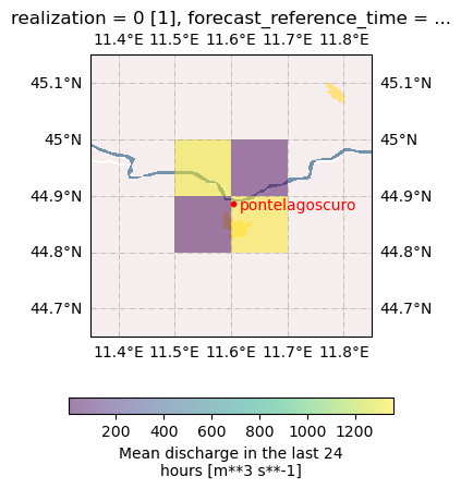
All is good. It is exactly where it should be. Note: the 4 pixels are the model grid cells.
Let’s read the data in memory, converting it to Xarray Dataset, then compute some statistics for the climatology, and extract the timeseries:
cl = climatology.to_xarray().chunk({"time":500})
seas = seasonal.to_xarray()
wb = water_balance.to_xarray()

# daily climatology
cmean = cl.groupby("time.dayofyear").mean()
cmin = cl.groupby("time.dayofyear").min()
cmax = cl.groupby("time.dayofyear").max()

# drop 29th of February, extract timeseries
cmax = cmax.where(cmax.dayofyear != cmax.dayofyear[59], drop =True).sel(latitude=ps['lat'],longitude=ps['lon'],method="nearest")
cmin = cmin.where(cmin.dayofyear != cmin.dayofyear[59], drop =True).sel(latitude=ps['lat'],longitude=ps['lon'],method="nearest")
cmean = cmean.where(cmean.dayofyear != cmean.dayofyear[59], drop =True).sel(latitude=ps['lat'],longitude=ps['lon'],method="nearest")

cmean["time"] =  pd.date_range("2022-01-01","2022-10-31")
cmin["time"]=  pd.date_range("2022-01-01","2022-10-31")
cmax["time"] =  pd.date_range("2022-01-01","2022-10-31")


wbdf = wb.sel(latitude=ps['lat'],longitude=ps['lon'], method="nearest").to_dataframe().reset_index()
wbdf.drop(["latitude", "longitude"], axis=1, inplace=True)
wbdf= wbdf[(wbdf.time.dt.month >= 1) & (wbdf.time.dt.month <= 12) ]
wbdf['time'] =  pd.DatetimeIndex(wbdf.time)
seas_df = seas.sel(lat=ps['lat'],lon=ps['lon'], method="nearest").to_dataframe()
seas_df = seas_df.drop(['lat','lon'], axis=1).reset_index()

# Since I don't want to plot every day of the forecast, filter weekly:
seas_df_w = seas_df[seas_df.time.dt.day.isin([2,9,16,23])]
leadtimes = seas_df_w.leadtime.dt.days.unique()
seas_df_w = seas_df_w.drop(["leadtime"], axis= 1)
seas_df_wf = seas_df_w.loc[(seas_df_w.time.dt.month >= 1) & ( seas_df_w.time.dt.month <= 12)].reset_index(drop=True)
seas_df_wf['time'] = pd.DatetimeIndex(seas_df_wf.time)
seas_df_wf['time'] = seas_df_wf.time.dt.strftime("%Y-%m-%d")
cmeanvals = cmean.dis24.values.T
cmaxvals = cmax.dis24.values.T
cminvals = cmin.dis24.values.T
Finally let’s plot the forecasts:
plot_seasonal(wbdf,
             seas_df_wf,
             clims = [cmeanvals,cmaxvals,cminvals],
             leadtimes = leadtimes,
             clim_range_y = ["2000","2021"],
             time_range = ["2022-01-01","2022-12-31"],
             figsize = (15,25))